Conventions

We use $σ$ to represent a binary digit, its subtitle usually refers to the position of a given binary digit inside a number (bit string).

In computing, bit numbering (or sometimes bit endianness) is the convention used to identify the bit positions in a binary number or a container of such a value. The bit number starts with zero and is incremented by one for each subsequent bit position. See also Bit numbering((Bit endianness)).

There are two different representation orders of a bit string:

• Least significant bit 0 bit numbering
• Most significant bit 0 bit numbering

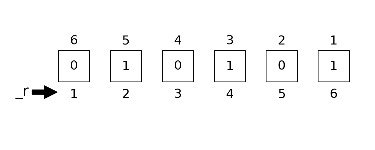
LSB 0 bit numbering

This follows the order of BitArray or other array representation of bits, e.g

For number 0b011101 (29)

See also LSB 0 bit numbering

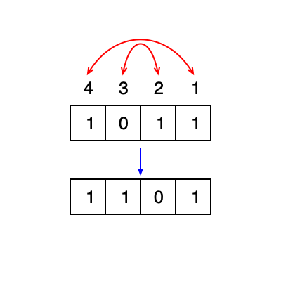
MSB 0 bit numbering

This follows the order of binary literal 0bxxxx, e.g

For number 0b011101 (29)

See also MSB 0 bit numbering.

Integer Representations

We use an Int type to store bit-wise (spin) configurations, e.g. 0b011101 (29) represents the configuration

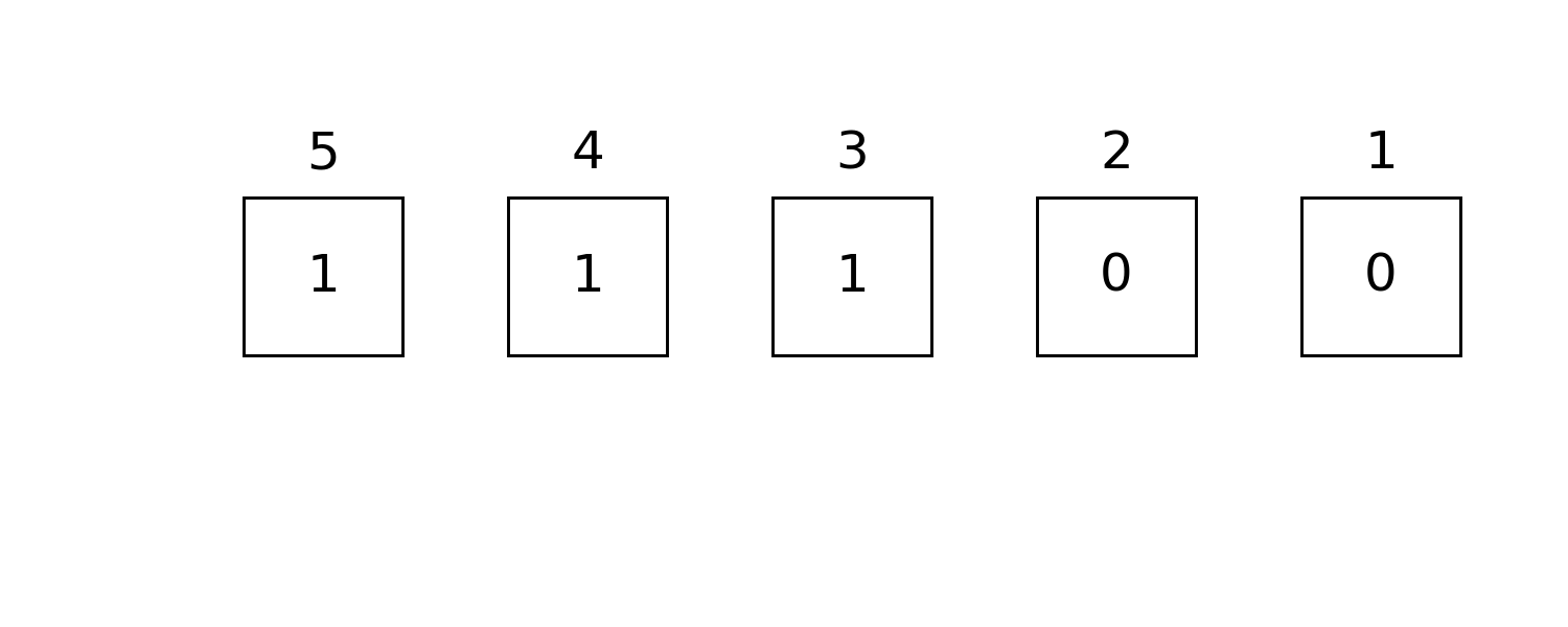
so we annotate the configurations $\vec σ$ with integer $b$ by $b = \sum\limits_i 2^{i-1}σ_i$. 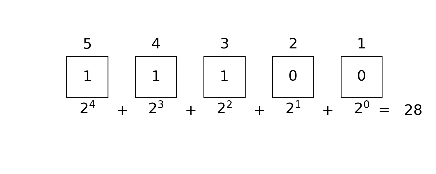e.g. we can use a number 28 to represent bit configuration 0b11100

julia> bdistance(0b11100, 0b10101) == 2  # Hamming distance
true

julia> bit_length(0b11100) == 5
true

In BitBasis, we also provide a more readable way to define these kind of objects, which is called the bit string literal, most of the integer operations and BitBasis functions are overloaded for the bit string literal.

We can switch between binary and digital representations with

• bitarray(integers, nbits), transform integers to bistrings of type BitArray.
• packabits(bitstring), transform bitstrings to integers.
• baddrs(integer), get the locations of nonzero qubits.

julia> bitarray(4, 5)
5-element BitArray{1}:
 false
 false
  true
 false
 false

julia> bitarray([4, 5, 6], 5)
5×3 BitArray{2}:
 false   true  false
 false  false   true
  true   true   true
 false  false  false
 false  false  false

julia> packbits([1, 1, 0])
3

julia> bitarray([4, 5, 6], 5) |> packbits;

A curried version of the above function is also provided. See also bitarray.

Bit String Literal

bit strings are literals for bits, it provides better view on binary basis. you could use @bit_str, which looks like the following

julia> bit"101" * 2
1010 ₍₂₎

julia> bcat(bit"101" for i in 1:10)
101101101101101101101101101101 ₍₂₎

julia> repeat(bit"101", 2)
101101 ₍₂₎

julia> bit"1101"[2]
0

to define a bit string with length. bit"10101" is equivalent to 0b10101 on both performance and functionality but it store the length of given bits statically. The bit string literal offers a more readable syntax for these kind of objects.

Besides bit literal, you can convert a string or an integer to bit literal by bit, e.g

julia> BitStr{5}(0b00101)
ERROR: MethodError: no method matching BitStr{5,T} where T(::UInt8)
Closest candidates are:
  BitStr{5,T} where T(::T<:Number) where T<:Number at boot.jl:741
  BitStr{5,T} where T(!Matched::Float16) where T<:Integer at float.jl:71
  BitStr{5,T} where T(!Matched::Complex) where T<:Real at complex.jl:37
  ...

Bit Manipulations

readbit and baddrs

julia> readbit(0b11100, 2, 3) == 0b10  # read the 2nd and 3rd bits as `x₃x₂`
true

julia> baddrs(0b11100) == [3,4,5]  # locations of one bits
true

bmask

Masking technic provides faster binary operations, to generate a mask with specific position masked, e.g. we want to mask qubits 1, 3, 4

julia> mask = bmask(UInt8, 1,3,4)
0x0d

julia> bit(mask; len=4)
┌ Warning: `bit(b; len)` is deprecated, use `BitStr{len}(b)` instead.
│   caller = ip:0x0
└ @ Core :-1
ERROR: MethodError: no method matching BitStr{4,T} where T(::UInt8)
Closest candidates are:
  BitStr{4,T} where T(::T<:Number) where T<:Number at boot.jl:741
  BitStr{4,T} where T(!Matched::Float16) where T<:Integer at float.jl:71
  BitStr{4,T} where T(!Matched::Complex) where T<:Real at complex.jl:37
  ...

allone and anyone

with this mask (masked positions are colored light blue), we have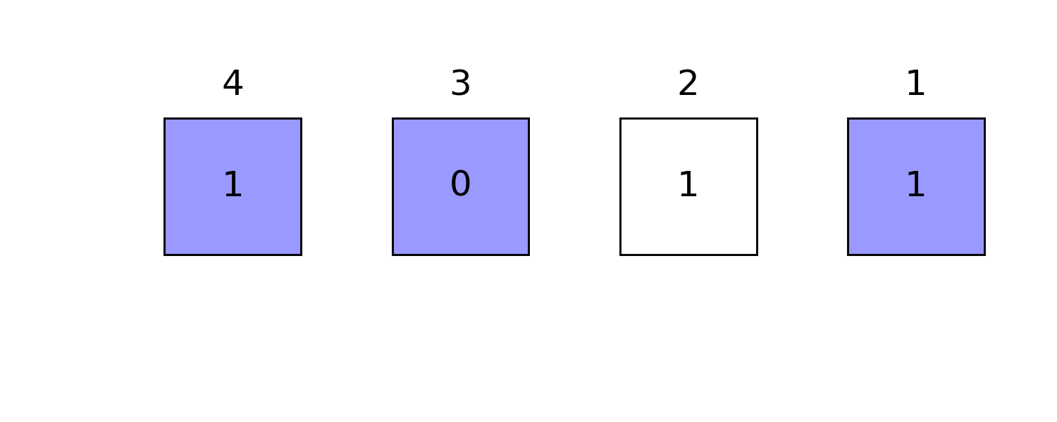

julia> allone(0b1011, mask) == false # true if all masked positions are 1
true

julia> anyone(0b1011, mask) == true # true if any masked positions is 1
true

ismatch

julia> ismatch(0b1011, mask, 0b1001) == true  # true if masked part matches `0b1001`
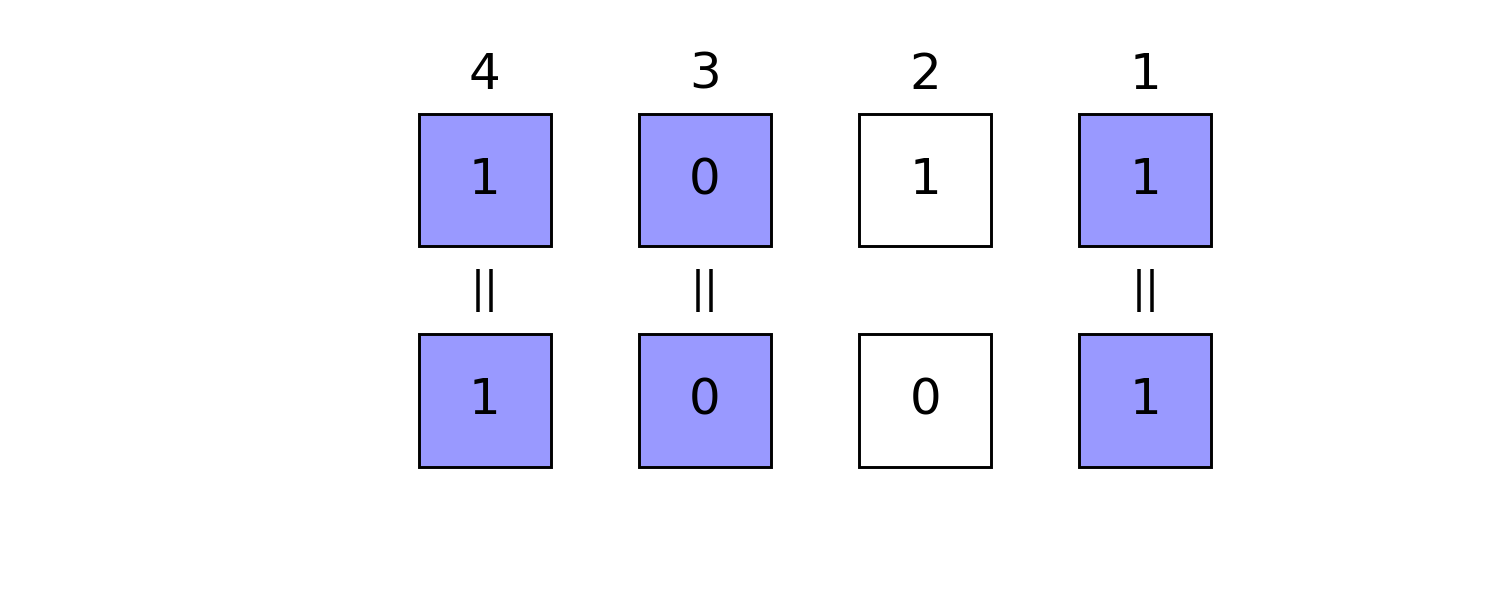
true

flip

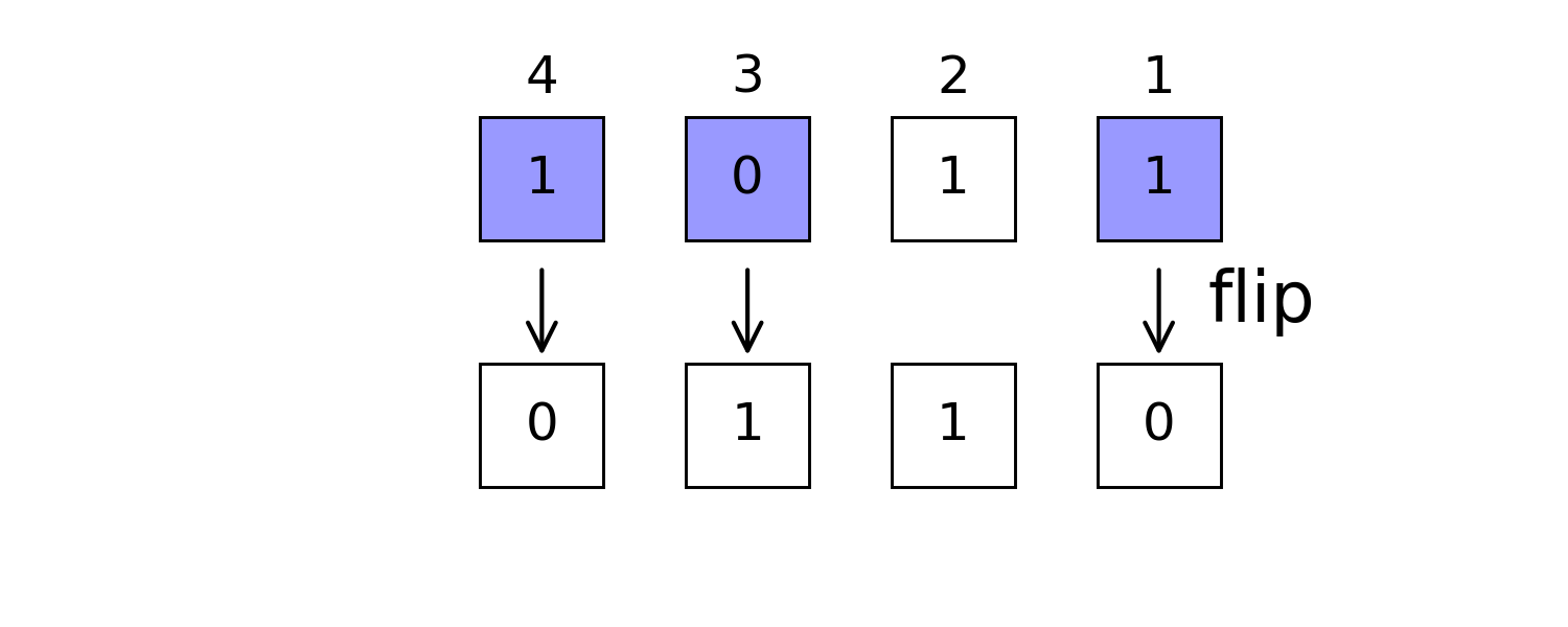
julia> bit(flip(0b1011, mask); len=4)  # flip masked positions
┌ Warning: `bit(b; len)` is deprecated, use `BitStr{len}(b)` instead.
│   caller = ip:0x0
└ @ Core :-1
ERROR: MethodError: no method matching BitStr{4,T} where T(::UInt8)
Closest candidates are:
  BitStr{4,T} where T(::T<:Number) where T<:Number at boot.jl:741
  BitStr{4,T} where T(!Matched::Float16) where T<:Integer at float.jl:71
  BitStr{4,T} where T(!Matched::Complex) where T<:Real at complex.jl:37
  ...

setbit

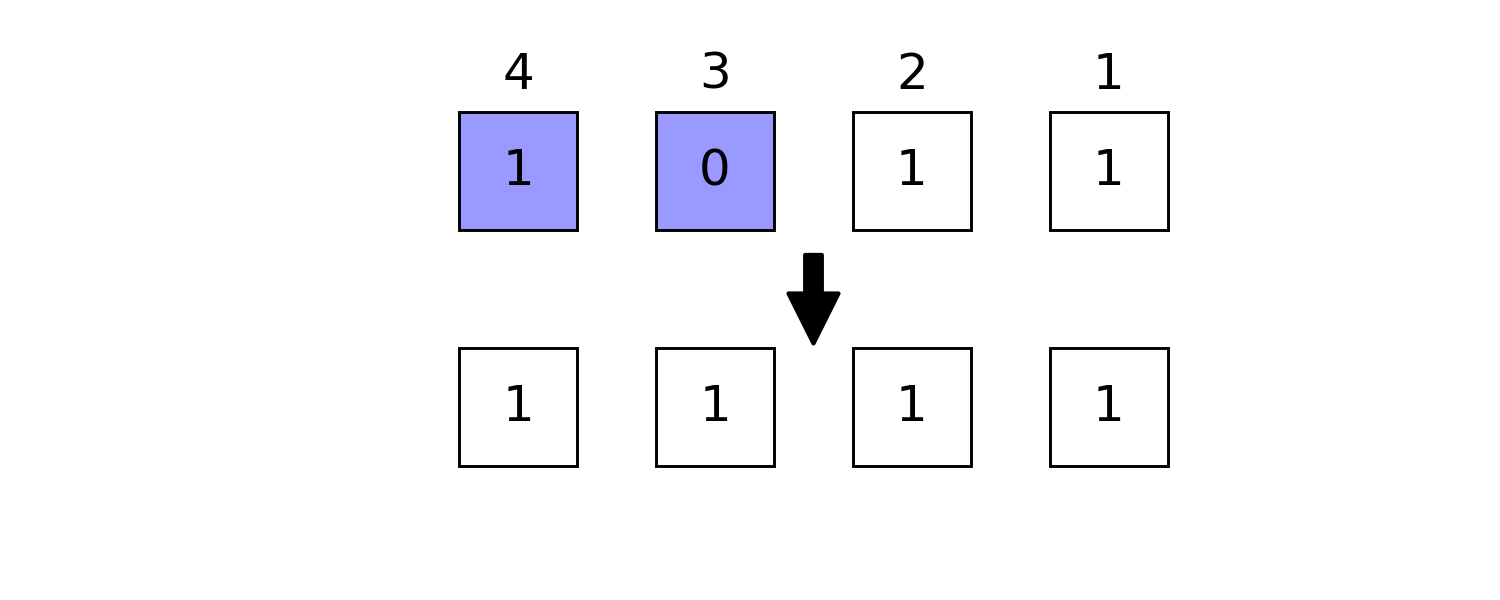
julia> setbit(0b1011, 0b1100) == 0b1111 # set masked positions 1
true

swapbits

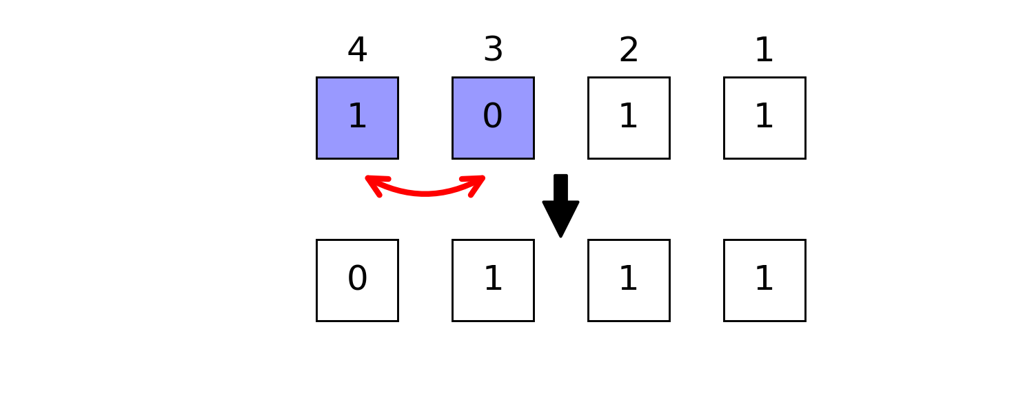
julia> swapbits(0b1011, 0b1100) == 0b0111  # swap masked positions
true

neg

julia> neg(0b1011, 2) == 0b1000
true

btruncate and breflect

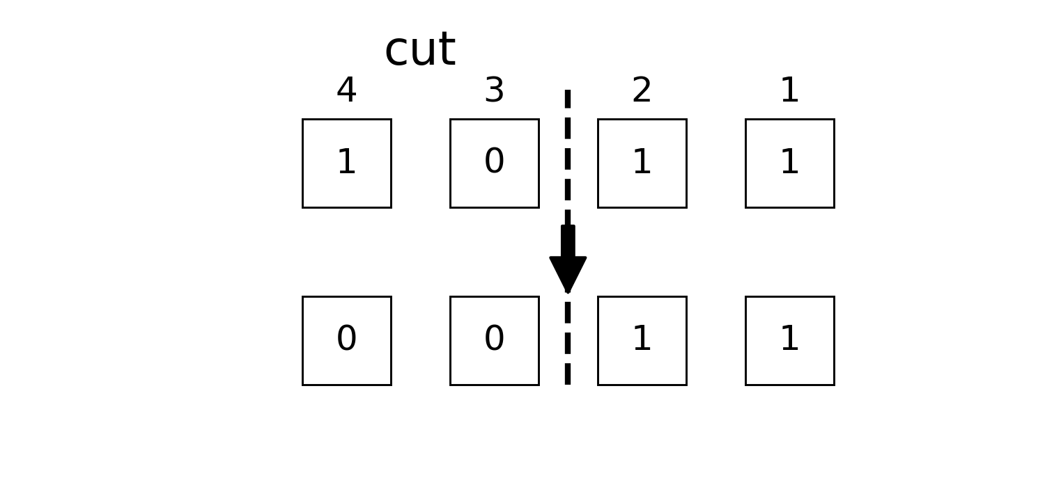
julia> btruncate(0b1011, 2) == 0b0011  # only the first two qubits are retained
true

breflect

julia> breflect(4, 0b1011) == 0b1101  # reflect little end and big end
┌ Warning: `breflect(nbits::Int, b::Integer)` is deprecated, use `breflect(b; nbits=nbits)` instead.
│   caller = top-level scope at none:0
└ @ Core none:0
true

For more detailed bitwise operations, see manual page BitBasis.

Number Readouts

In phase estimation and HHL algorithms, one need to read out qubits as integer or float point numbers. A register can be read out in different ways, like

• bint, the integer itself
• bint_r, the integer with bits small-big end reflected.
• bfloat, the float point number $0.σ₁σ₂ \cdots σ_n$.
• bfloat_r, the float point number $0.σ_n \cdots σ₂σ₁$.

julia> bint(0b010101)
0x15

julia> bint_r(0b010101, nbits=6)
0x2a

julia> bfloat(0b010101)
0.65625

julia> bfloat_r(0b010101, nbits=6);

Notice the functions with _r as postfix always require nbits as an additional input parameter to help reading, which is regarded as less natural way of expressing numbers.

Iterating over Bases

Counting from 0 is very natural way of iterating quantum registers, very pity for Julia

julia> itr = basis(4)
0:15

julia> collect(itr)
16-element Array{Int64,1}:
  0
  1
  2
  3
  4
  5
  6
  7
  8
  9
 10
 11
 12
 13
 14
 15

itercontrol is a complicated API, but it plays an fundamental role in high performance quantum simulation of Yao. It is used for iterating over basis in controlled way, its interface looks like

julia> for each in itercontrol(7, [1, 3, 4, 7], (1, 0, 1, 0))
           println(string(each, base=2, pad=7))
       end
0001001
0001011
0011001
0011011
0101001
0101011
0111001
0111011

Reordering Basis

We store the wave function as $v[b+1] := \langle b|\psi\rangle$. We are able to reorder the basis as

julia> v = onehot(5, 0b11100)  # the one hot vector representation of given bits
32-element Array{Float64,1}:
 0.0
 0.0
 0.0
 0.0
 0.0
 0.0
 0.0
 0.0
 0.0
 0.0
 ⋮
 0.0
 0.0
 0.0
 0.0
 0.0
 1.0
 0.0
 0.0
 0.0

julia> reorder(v, (3,2,1,5,4)) ≈ onehot(5, 0b11001)
true

julia> invorder(v) ≈ onehot(5, 0b00111)  # breflect for each basis
true